Augmented Reality in Python

This was a project in ENPM673: Perception for Autonomous Robots at the University of Maryland. Unlike some of the other projects I’ve written about (most of which spanned at least a half semester or longer), this project was completed in about 2 weeks. I would be remiss in this writeup if I did not acknowledge the contributions of my partner in this project, Justin Albrecht, without whom this project would not have been possible. He deserves significant credit for the ideation and execution of this project.

The Task

We were given 3 videos containing 1-3 custom Augmented Reality (AR) tags. We were tasked with tracking these tags through the video, identifying them based on their geometry, and superposing both images and cubes on top of them. We were not allowed to use cv2.FindHomography, cv2.warpPerspective, or any similar one line solutions.

The original videos are not particularly interesting. You can watch them below to get a sense of what we were working with.

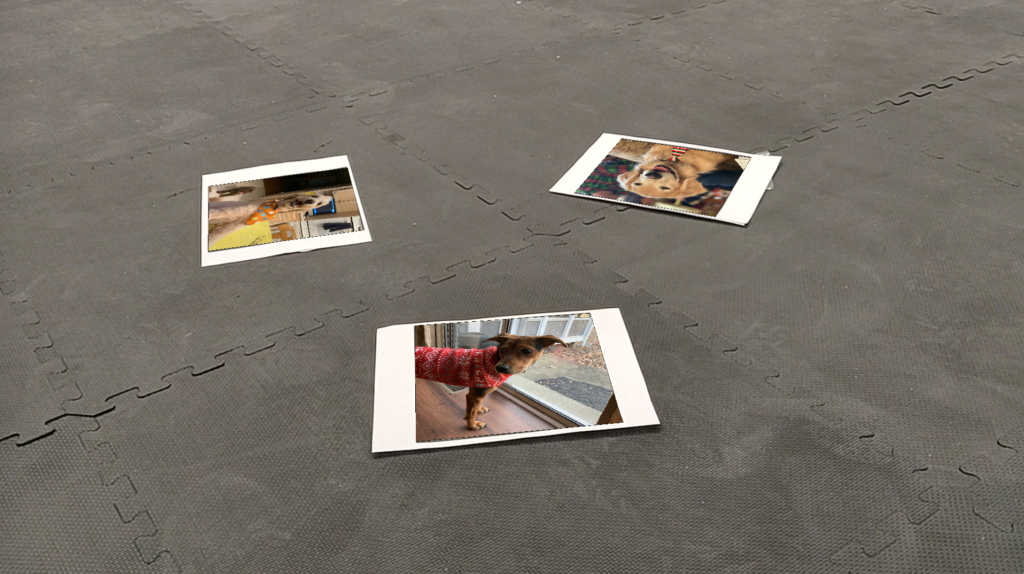
We chose to use photos of some of the dogs in our families. We hope these photos bring you even a fraction of the joy that they bring us.

AR Tags

The idea behind AR tags is fairly simple. Their high contrast, square geometry makes them relatively easy to detect and track in an image. Each tag has its own “right way up”, so they encode orientation. The squares that comprise the tag also identify it uniquely via a binary string, so they also encode their own identity.

A sample AR tag, divided into an 8×8 grid for analysis

You could use an AR tag to identify surfaces or locations for a robot to navigate to.

Corner Detection

Initial Filtering

We evaluated each video one at a time. Within each video, we worked frame by frame, treating each frame as an individual static image. We first converted the frame to a greyscale color space. We experimentally determined the ideal grayscale threshold that made just the AR tag clearly visible in the frame and eliminated all undesired image elements.

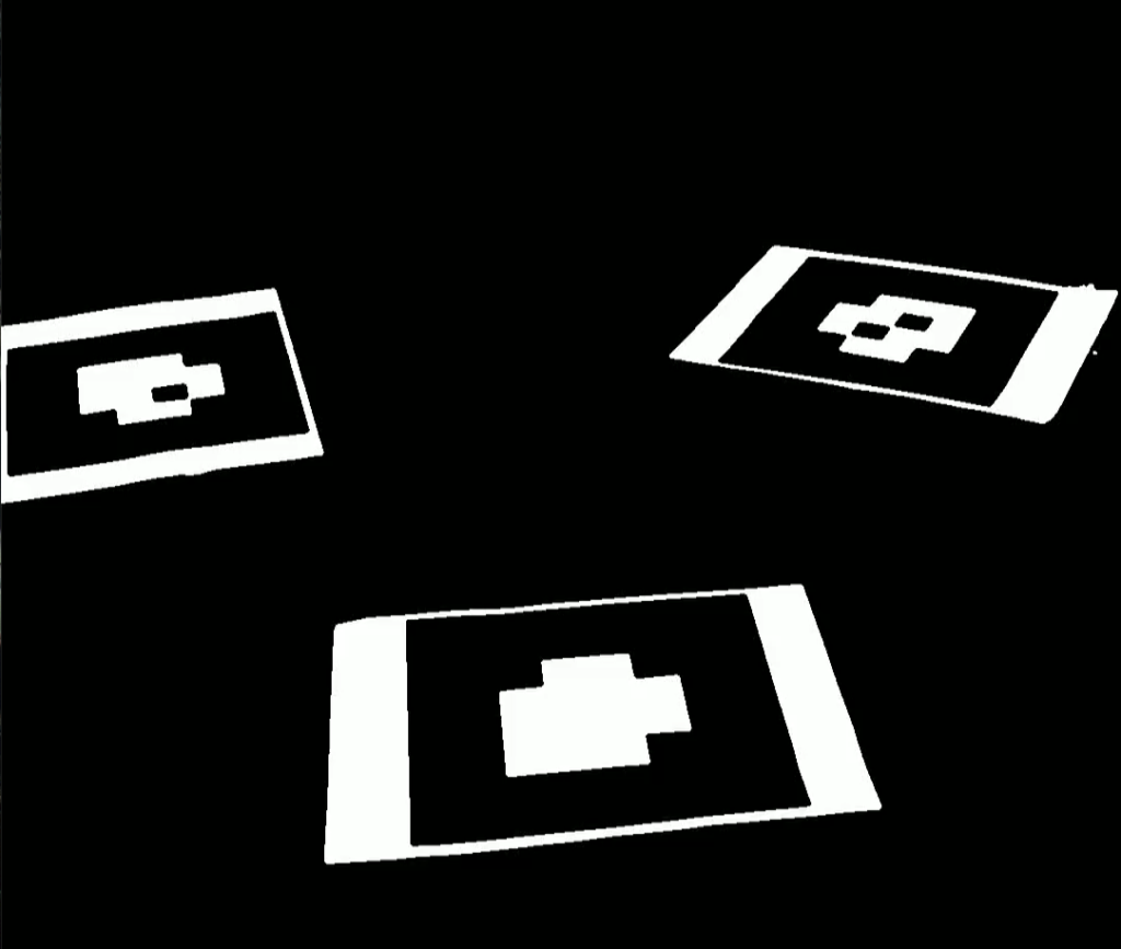
Example photo showing the result of a binary threshing

You can view a threshed version of the video here:

If you watch this video closely, you’ll see some of the motion blur artifacts that made some frames more challenging to analyze. Note how the inner squares of the tag change shape and size as the video progresses.

Contour Detection and Filtering

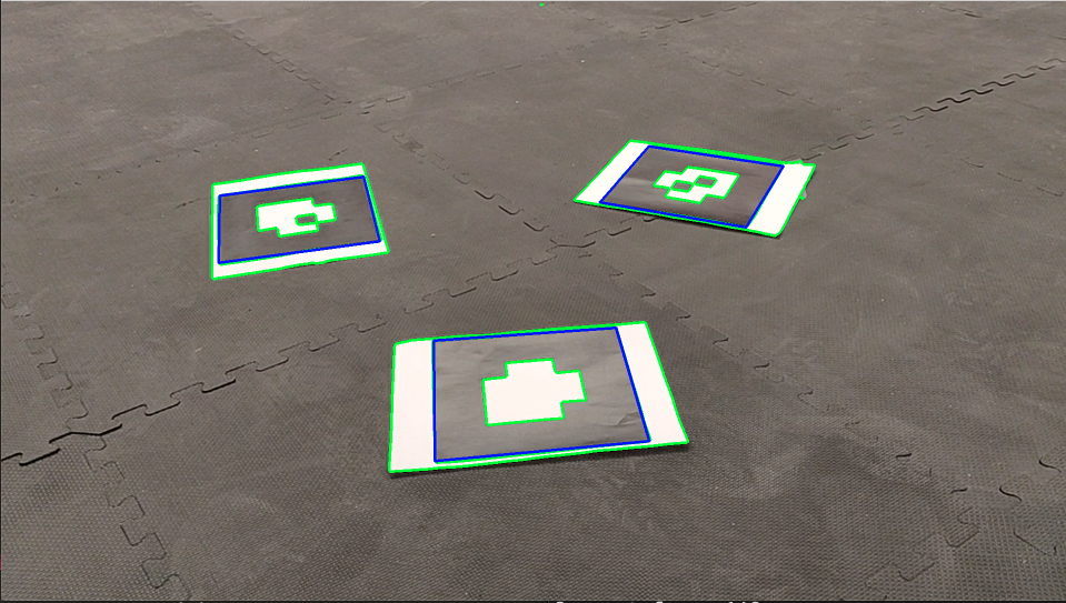
On the binary image we call cv2.findContours. This function returns both the list of all contours in the image as well as their hierarchical relationship. Using the hierarchical relationship, we filter out any contours that do not have a parent or child contour. By further filtering these contours so that only the largest 3 remain, we reduce most noise and erroneous contours. This leaves us with only the contours that are associated with the black region of the AR tag. The image below shows, in green, all of the contours that are found in the image, and, in blue, only the contours that remain after filtering.

Getting Corners

After the contours have been filtered so that only the edges of the black region of the tag remain we call the our function approx_quad on the contour. This takes in the contour and tries to approximate the region as a quadrilateral. Using the function approx_quad and filtering for only polygons that have four sides we can ensure that we have found the corners of the tag. We store the corners in a python list of lists called corners, where the length of corners will be equal to the number of detected tags a given frame. Inside each element of corners is a list of four points that correspond to the corners. approx_quad orders the corners so that they are arranged counter-clockwise, but the starting corner may change from frame to frame.

Decoding

After we have defined the corners of the black region of the tag we need to use homography to warp the image from the camera coordinate frame into a square coordinate frame that will allow us to decode the tag.

Homography Computation

To find a homography matrix that will allow us to convert between our camera cordinates and the square coordinates we need eight points. Four of the points are the corners of the tag that we have from detection. The other four points are the corners of our square destination image. The dimensions of the destination are somewhat arbitrary but if it is too large we will start to have holes, since there are not enough pixels in the source image, and if it is too small we will have a lower resolution and will start to lose information. To fix this we found the number of pixels that were contained within the four corners of the tag and took the square root of that number to get an ideal dimension $dim$. The four corners are then [(0,0), (0, $dim$), ($dim$, $dim$), ($dim$, 0)]

Now that we have the eight points we can generate the A matrix below:

\begin{equation} A =\begin{bmatrix} -x_1 & -y_1 & -1 & 0 & 0 & 0 & x_1*xp_1 & y_1*xp_1 & xp1\\ 0 & 0 & 0 & -x_1 & -y_1 & -1 & x_1*yp_1 & y_1*yp_1 & yp1\\ -x_2 & -y_2 & -1 & 0 & 0 & 0 & x_2*xp_2 & y_2*xp_2 & xp2\\ 0 & 0 & 0 & -x_2 & -y_2 & -1 & x_2*yp_2 & y_2*yp_2 & yp2\\ -x_3 & -y_3 & -1 & 0 & 0 & 0 & x_3*xp_3 & y_3*xp_3 & xp3\\ 0 & 0 & 0 & -x_3 & -y_3 & -1 & x_3*yp_3 & y_3*yp_3 & yp3\\ -x_4 & -y_4 & -1 & 0 & 0 & 0 & x_4*xp_4 & y_4*xp_4 & xp4\\ 0 & 0 & 0 & -x_4 & -y_4 & -1 & x_4*yp_4 & y_4*yp_4 & yp4\\ \end{bmatrix} \end{equation}

From this A matrix we can solve for the vector $h$, which is the solution to:
\begin{equation}
Ah=0
\end{equation}

By reshaping our vector $h$, we can find the homography matrix:

\begin{equation}
H =\begin{bmatrix}
h_{1} & h_{2} & h_{3} \\
h_{4} & h_{5} & h_{6} \\
h_{7} & h_{8} & h_{9} \\
\end{bmatrix}
\end{equation}

To solve for the vector $h$, we can use Singular Value Decomposition or SVD. This will decompose our $A$ matrix into three matrices, $U$, $\Sigma$, and $V$.

To perform the decomposition the following steps need to be followed:

Find eigenvectors $(w_i)$ and eigenvalues $(\lambda_i)$ for $A^TA$.
Sort $\lambda_i$ from largest to smallest
Compose $V$ as an $n\times n$ matrix such that the columns are $w_i$ in the order of sorted $\lambda_i$
Create the list of singular values $(\sigma_i)$ from the square root of the non-zero $\lambda_i$. $\sigma_i=\sqrt{\lambda_i}$
Compose $\Sigma$ as an $m \times n$ matrix where the $i$th diagonal element is $\sigma_i$ and all other elements are zero.
Use the relationship $Av_i=\sigma_iu_i$ to solve for the columns of $U$.

Note:
$v_i$ is the columns of $V$
$u_i$ is the columns of $U$

Using the steps above, we can decompose $A$ into $U$, $\Sigma$, $V$.

After this decomposition we know that our $h$ vector can be approximated by the column of $V$ that corresponds with the small singular value in $\Sigma$. Since the singular values are ordered from largest to smallest, $h$ can be approximated as the last column of $V$

\begin{equation}
h = V[:,-1]
\end{equation}

Creating the Square Image

After we have computed the homography matrix we need to generate a new set of points in the square frame, and then create a new image using the pixels from source image but in their new location. For any point in the camera coordinates $X^c$ ($x$,$y$), we can compute that point in the square coordinates $X^s$ ($x’$,$y’$), using the following equations:

\begin{equation} \label{homography}
sX^s =
\begin{bmatrix} sx’ \ sy’ \ s \ \end{bmatrix}
= H
\begin{bmatrix} x \ y \ 1 \ \end{bmatrix}
\end{equation}

\begin{equation}
x’ = \frac{sX^s[0]}{sX^s[2]}
\end{equation}

\begin{equation}
y’ = \frac{sX^s[1]}{sX^s[2]}
\end{equation}

We can generate new points for all ($x$,$y$) in a given frame. The points generated are floats with multiple decimal places. There are several possible approaches to remedy this, including averaging the pixel values around the closest four pixels, picking the closest neighbor, or even simply truncating the floating point value as an integer. We decided to use this last approach for its simplicity and because the grid size of the tags is so large compared to any pixel that it this loss of resolution does not affect the decoding of the tag.

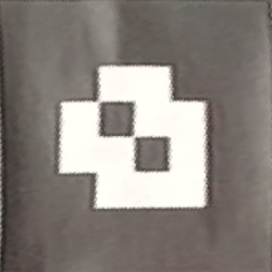
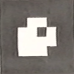
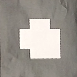
It is also important to note that any points outside of the boundaries of the corners of the tag will be outside of the dimensions of our destination image. We can generate a new image by taking only the points that lie in the range of our destination image and reconstruct an image pixel by pixel in the new coordinates. The resulting images looks like this:

Decoding the Tag into a Binary Matrix

Now that we have each of the tags as a square image we can start the process of decoding them into a binary matrix. We know that the tag is made up of an 8×8 grid so we divide the square into 64 sectors and create a new matrix that is 0 if that sector is black and 1 if that sector is white. In order to determine if the sector is black or white, we threshold the square image using an experimentally determined value into a binary image. We then take the mean of that sector and if the mean is closer to 0, then the value for that sector is 0 and if the mean is closer to 255, the value for that sector is 1.

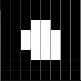
The process above gives the example 8×8 binary matrix shown below:

\begin{equation}
\begin{bmatrix}
0 & 0 & 0 & 0 & 0 & 0 & 0 & 0\\
0 & 0 & 0 & 0 & 0 & 0 & 0 & 0\\
0 & 0 & 0 & 1 & 1 & 0 & 0 & 0\\
0 & 0 & 1 & 1 & 1 & 1 & 0 & 0\\
0 & 0 & 1 & 1 & 1 & 1 & 0 & 0\\
0 & 0 & 0 & 1 & 1 & 1 & 0 & 0\\
0 & 0 & 0 & 0 & 0 & 0 & 0 & 0\\
0 & 0 & 0 & 0 & 0 & 0 & 0 & 0
\end{bmatrix}
\end{equation}

Decoding the Orientation and Tag ID

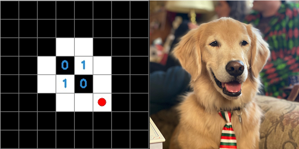
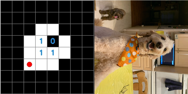
Now that we have a data structure for the information on the tag it is possible to determine both the orientation of the tag and the tag ID. The orientation is determined by a white square in any of the zero indexed positions [2,2], [5,2], [5,5], [2,5]. The ID is then derived from the inner four sectors of the tag and is composed of a four character string made up of ones and zeros. The order of characters is counter-clockwise and the first character is defined by the sector opposite the corner that defines the orientation. The images below show a red circle in the sector that defines the rotation and the resulting tag ID.

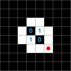
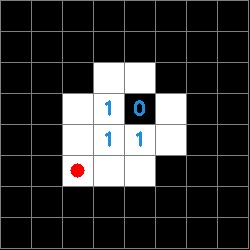
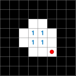
To determine the tag ID, we look the inner 4 elements of our square binary matrix.

\begin{equation}
\begin{bmatrix}
0 & 0 & 0 & 0 & 0 & 0 & 0 & 0\\
0 & 0 & 0 & 0 & 0 & 0 & 0 & 0\\
0 & 0 & 0 & 1 & 1 & 0 & 0 & 0\\
0 & 0 & 1 & 1 & 0 & 1 & 0 & 0\\
0 & 0 & 1 & 1 & 1 & 1 & 0 & 0\\
0 & 0 & 1 & 1 & 1 & 0 & 0 & 0\\
0 & 0 & 0 & 0 & 0 & 0 & 0 & 0\\
0 & 0 & 0 & 0 & 0 & 0 & 0 & 0
\end{bmatrix}\rightarrow
\begin{bmatrix}
1 & 0\\\
1 & 1
\end{bmatrix}
\end{equation}

This is read counterclockwise with the start position determined by the orientation. In this example, the tag ID would be 0111.

Superposing an Image

After we have determined the position, orientation, and ID of all the tags in a given frame we can then superpose the tag with our images of dog. The steps to do this are as follows:

Match the tag ID to an image

The IDs of the three tags and their corresponding photos are hard coded at the start of the program. We simply check the tag ID string to see if it matches any of the existing tags and assign the new image to be its corresponding dog image. It would be trivial to add additional tags and photos to this system.

Rotate the image

The function we use to decode a tag returns a number of rotations necessary to match the rotation of the tag. This number is either 0, 1, 2, or 3. We can then apply either no rotation or a multiple of 90° to the dog image using the function cv2.rotate()

Use homography to generate a new image

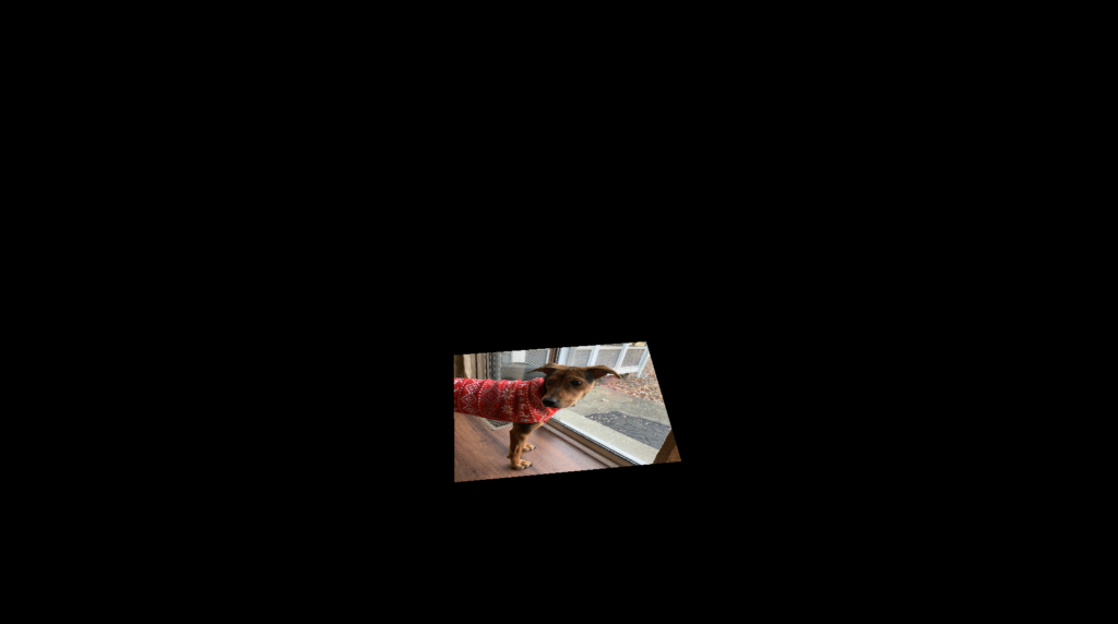
We then use the same process as above to generate a warped version of our dog image. In this case however instead of generating a square image of arbitrary size, we instead create an image that is the same size as the original frame. When we generate our new homography matrix we need to use the corners of the frame in addition to the corners of the tag. We can then follow the same process from the Homography section, to generate a new image that is the same size as our frame but has a warped image of the dog and is black everywhere outside of the frame.

Blank the original region of the tag

In order to perform the next step we need to blank the region of the image where the tag is. We can achieve this by drawing a filled black contour in the region defined by the corners of the tag. The output of drawing this contour is shown below:

Add the new image to the existing frame

Now that we have the image generated from homography and the original frame with the blank region we can use the function cv2.bitwise_or() to add them together. Since the first image is black (0) everywhere except the tag and the second image is black (0) only in the tag region, the output is the dog superposed onto the tag:

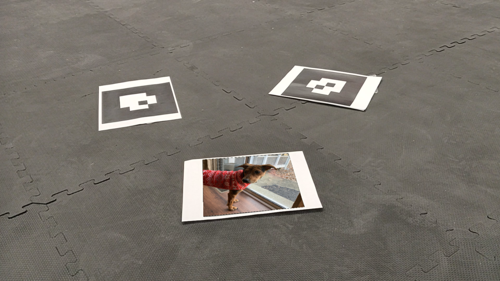
Repeating this for all three tags yields a cohesive image with all 3 dogs superposed:

Dog Videos

We produced several output videos for each input video. Here’s the simplest, 1 tag, 1 dog:

It’s interesting to look at the video with the contours shown. Here’s 1 tag, 1 dog, with contours:

I’m going to omit the other dog+contour videos for this section. If you want to see them, I’ll have them linked (instead of embedded) at the bottom of this page. Below are the videos for 2 and 3 tags.

Superposing a Cube

The coordinates of the corners of our cube, in the world frame, are:

\begin{equation}
\text{Corners}_{w}=\begin{bmatrix}
x_1, & y_1, &0 \\
x_2, & y_2, &0 \\
x_3, & y_3, &0 \\
x_4, & y_4, &0 \\
x_1, & y_1, & -d\\
x_2, & y_2, & -d \\
x_3, & y_3, & -d \\
x_4, & y_4, & -d \\
\end{bmatrix}
\end{equation}

where $d$ is the height of the cube. The base of the cube is flush with the floor plane of the world frame, so the first four points have zero $\hat{Z}$ component. The last four points bound the top face of the cube, and exist $d$ away from the floor plane. Our task is to find these points in the image frame so that they can be displayed in the image.

At the start, all we know are the coordinates of our tag corners in the camera frame:

\begin{equation}
\text{Corners}_{c}=\begin{bmatrix} x_{c_1}, & y_{c_1}\\
x_{c_2}, & y_{c_2}\\
x_{c_3}, & y_{c_3}\\
x_{c_4}, & y_{c_4}\\
\end{bmatrix}
\end{equation}

as well as the camera intrinsic matrix (provided):

\begin{equation}
K=\begin{bmatrix}
1406.084 &0&0\\
2.207 & 1417.999& 0\\
1014.136 & 566.348& 1
\end{bmatrix}
\end{equation}

We start by computing the homography transform ($H$) that converts our points from the image frame (skewed) to the world frame (square). This is the same computation done earlier to make our tags square for identification. We use this to convert the tag corners (the base of our cube-to-be) from the image frame to the world frame. This gets us the first four points of $\text{Corners}_w$. The other four corners (the top face of our cube) are those same points just shifted by $-d$. In the world frame, the Z axis points into the floor, so this negative is necessary to make the cube exist above the floor plane. We now need to convert the coordinates from the camera frame back to the world frame. To do this, we’ll need the Projection Matrix ($P$).

Finding the Projection Matrix

\begin{equation}
P=K\begin{bmatrix}
R & | & t
\end{bmatrix}
\end{equation}

To get $P$, we need to evaluate all of the components and sub-components that it is comprised of.

\begin{equation}
H=K\widetilde{B}
\end{equation}

\begin{equation}
B=\widetilde{B}(-1)^{|\widetilde{B}|<0}
\end{equation}

\begin{equation}
B=\begin{bmatrix}
b_1 & b_2 & b_3
\end{bmatrix}
\end{equation}

\begin{equation}
H=\begin{bmatrix}
h_1 & h_2 & h_3
\end{bmatrix}
\end{equation}

\begin{equation}
\lambda=\begin{pmatrix}
\frac{||K^{-1}h_1||+||K^{-1}h_2||}{2}
\end{pmatrix}^{-1}
\end{equation}

\begin{equation}
r_1=\lambda b_1
\end{equation}

\begin{equation}
r_2=\lambda b_2
\end{equation}

\begin{equation}
r_3=r_1\times r_2
\end{equation}

\begin{equation}
t=\lambda b_3
\end{equation}

\begin{equation}
R=\begin{bmatrix}
r_1 & r_2 & r_3
\end{bmatrix}
\end{equation}

Generating Top Corner Points

We then use the projection matrix $P$ to convert these new points from the world frame to the image frame, where they can be superposed on the image. To do this, we start with our homogeneous coordinates for the bottom corners, $X_{c1}$, in the camera frame:

\begin{equation}
X_{c1}=\begin{bmatrix}
x_1 & x_2 & x_3 & x_4\\
y_1 & y_2 & y_3 & y_4\\
1 & 1 & 1 & 1
\end{bmatrix}
\end{equation}

These become scaled homogeneous coordinates in the world frame:

\begin{equation}
sX_s=H\cdot X_{c1}
\end{equation}

\begin{equation}
sX_s=
\begin{bmatrix}
sx’\\
sy’\\
s
\end{bmatrix}
\end{equation}

We need to normalize these so the last row is 1:
\begin{equation}
X_s=\frac{sX_s}{sX_s[2]}
\end{equation}
Where $sX_s[2]$ is the 3rd (0 index) row of $sX_s$

\begin{equation}
X_w=\begin{bmatrix}
X_s[0]\\
X_s[1]\\
-d\\
1
\end{bmatrix}
\end{equation}

Now that we have shifted the points in $z$ in the world frame we need to use the projection matrix $P$ to get the top corners $X_{c2}$ back in camera coordinates.

\begin{equation}
sX_{c2}=P\cdot X_w
\end{equation}

\begin{equation}
X_{c2}=\frac{sX_{c2}}{sX_{c2}[2]}
\end{equation}

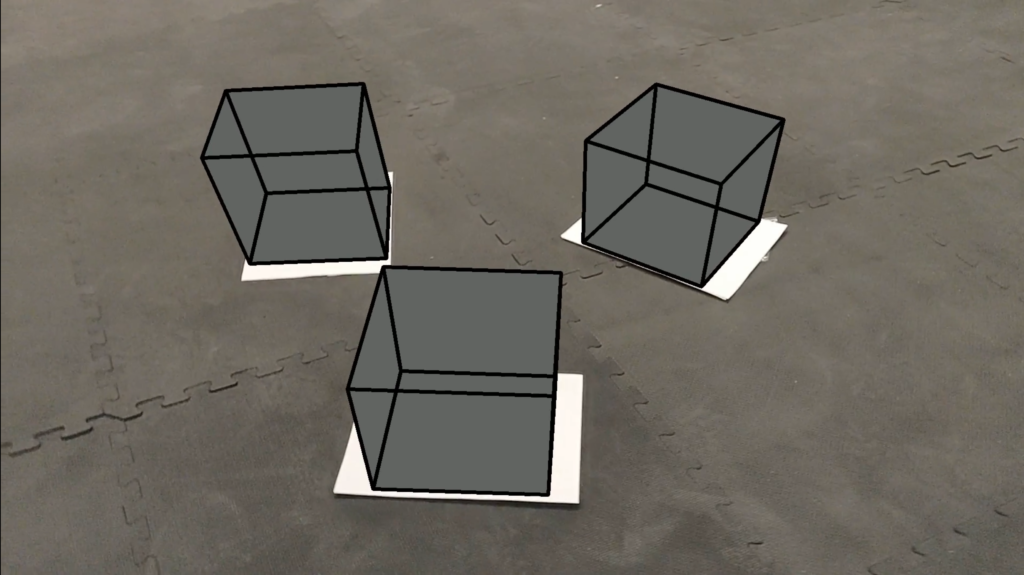
Drawing Lines and Contours

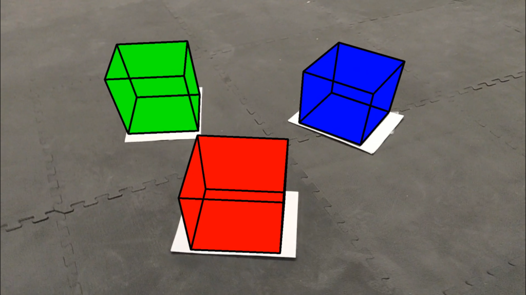
Once we have the corner points, we use cv2.drawContours and cv2.line to create first the faces and then the edges of our cubes. This creates the shaded wire-frame aesthetic that characterizes our project.

Monochromatic cubes rendered on their tags

Cube faces can also be colored to correspond to their unique tag IDs:

Colored cubes rendered on their specific tags

Cube Videos

Just like with the dog videos, we produced several different video combinations. I’ve embedded the simplest three here – a video with 1, 2, and 3 tags (and cubes). The other videos (with contours) will be appended at the end of this page.

Dogs and Cubes

We modified our program so you could run Dog_mode and Cube_Mode concurrently.

Smoothing

Go back and watch at least one of those cube videos. Notice how jittery the cubes are. Due to noise and blur in the video, the base of our cubes (and then also their top points), shift considerably from frame to frame. This is most obvious in the threshed video at the top of the page. Here it is again (to save you from scrolling all that way):

Watch the edges of the tags as the video goes. Notice how they shift about. That’s the core cause of our jittery cubes. We wanted to improve these outputs by applying a smoothing or filtering function to the cubes.

Initial Efforts – Frame Interpolation

We initially attempted to smooth the video by interpolating additional frames to create a video with a higher effective frame rate. We took two frames, and created 10 blended frames, each 10% more of the next (N) frame and 10% less of the original (O) frame. In this way, each pair of the original video frames became 12 new frames (the original, 90%O+10%N, 80%O+20%N …, 10%O+90%N, and the next). This produced smoother video motion, but didn’t aid in the cube jitter issue.

Improved Smoothing – Interframe Averaging

We then moved to our final smoothing solution. Unlike in the original videos, which processed the video frame by frame as it was read from the file, this attempt started by reading in the entire video into an array of frames. This resolved a tricky issue with video.set() which does not permit backtracking. We later abandoned this resource intensive approach for a simpler one – we now read in the first few frames (however many are needed to get started) and then read in only the “frontier” frame for each successive iteration.

Using a look-ahead and look-behind method, we average the corner coordinates for the top and bottom of the cube with their positions over several previous and post frames. The computed average for each corner is used as the points for that frame. This process is repeated for all subsequent frames. As a check against undesired cube behavior, we examine this average and compare it with the original position. If the average is too far away from the original position, we assume there was some error (the wrong point averaged due to excessive motion/blur), and the original position is used instead. This smoothing function works for an arbitrary number of preceding and post frames, allowing for varying amounts of smoothing. The more frames that are averaged results in a smoother, less jittery cube, but may cause cube drift, where the cube position slides slightly from the tag due to camera movement in neighboring frames. Cube drift becomes more noticeable as the frame count increases. See the 15 frame smoothed videos in the Videos Section for examples of this.